Data Analytics for Beginners: Part 1

If you want more practice data projects, be sure to check out http://www.teamleada.com

What You Will Learn:

This post is meant for ANYONE interested in learning more about data analytics and is made so that you can follow along even with no prior experience in R. Some background in Statistics would be helpful (making the fancy words seem less fancy) but neither is it necessary. You will learn how to answer a question and discover new trends with a dataset by walking you through step by step in an example. You will complete a “data project” given from Kaggle, a data science competition website, and if you follow carefully, you can place yourself at the top 20% of all competitors.

Why You Should Follow Along:

Are you a professional looking to develop additional skills that will make you high demand in the job market? Do you lack “technical” skills and don’t want to dive into the black hole of computer science? In todays day and age, data analytics has become a business problem. Almost all decisions are now based upon metrics instead of intuition. Whether you are A/B testing, segmenting customers, or predicting stock prices, you are using analytics to do so. We believe that following the agricultural and industrial revolutions is the information revolution, and unique from the plow or the assembly line, the key to this revolution is the knowledge of how to analyze data.

Hal Varian, Chief Economist at Google, said this about the field of Data Analytics and Data Science:

If you are looking for a career where your services will be in high demand, you should find something where you provide a scarce, complementary service to something that is getting ubiquitous and cheap. So what’s getting ubiquitous and cheap? Data. And what is complementary to data? Analysis. So my recommendation is to take lots of courses about how to manipulate and analyze data: databases, machine learning, econometrics, statistics, visualization, and so on.

Who We Are:

We are recent UC Berkeley grads who studied Statistics (among other things) and realized two things: (1) how essential an understanding of Statistics and Data Analysis was to almost every industry and (2) how teachable these analytic practices could be.

Table of Contents:

Part 1:

1. Installing R and RStudio
2. Kaggle Data Project: Titanic – Machine Learning from Disaster
3. Data Exploration
4. Conclusion

Part 2:

1. Data Cleaning

Part 3:

1. Training a Model
2. Fitting a Model

Tips for following along

We recommend copying and pasting all code snippets that we have included, with the exception of the first one where you need to set your own working directory (this is explained later). While copying and pasting allows you to run the code, you should read through and have an intuitive understanding of what is happening in the code. Our goal isn’t to necessarily teach R syntax, but to provide a sense of the process of digging into data and allow you to use other resources to learn R.

Feel free to ask questions on our Kaggle Forum post and we will respond as soon as possible!

Installing R and Rstudio

If you haven’t yet, you will need to install R and RStudio. R is a useful and free application for data analytics that is widely used by statisticians and data miners. RStudio provides a more user friendly interface that will speed up your learning greatly!

Macs
Download and install R here: Mac Install

Windows
Download and install R here: Windows Install

Linux
Download and install R here: Linux Install

Next, choose the appropriate package for RStudio here: RStudio Install

Kaggle Data Project: Titanic – Machine Learning From Disaster

To have access to the data project, you also need to become a Kaggle Competitor, don’t worry it’s free! Sign up for Kaggle here.

The Kaggle competition asks you to predict whether a passenger survived the Titanic crash. You are given two datasets (Train & Test) each of which include predictor variables such as Age, Passenger Class, Sex, etc. With these two data sets we will do the following:

1. Create a model which will predict whether a passenger survived using only the Train data set
2. Predict whether the passengers survived in the Test data set based on the model we created

See the full description of the project here. The project result will be a spreadsheet with predictions for which passengers in the Test data set survived. The spreadsheet will have only two columns: a column for the Passenger ID and another column which indicates whether they survived (0 for death, 1 for survival).

Starting the Kaggle Data Project

Create a folder called “kaggle” on your desktop. Now download the datasets, train and test, here, and save it in the kaggle folder on your desktop.

In RStudio, we must first create a file for us to write in. Go to File ==> New ==> Rscript. Now in that file we must tell R where our current working directory is. We do this by using the setwd() function. Your working directory indicates to R which folder to look for the data you want to use, for us it will be the Train and Test files you downloaded from Kaggle. Remember everything in R you type is case sensitive!

For Mac Users:

setwd("/Users/your_user_name/Desktop/kaggle/")

Using the image above as an example the correct code would be:

setwd("/Users/Clair/Desktop/kaggle/")

For Windows users:

setwd("C:/Users/your_user_name/Desktop/kaggle")

Running your RCode

To run what you just wrote in your RScript, put your cursor on a line of code in your RScript and enter control and return at the same time! It should now pop up on the bottom left window labeled Console in blue and if there is no red code that follows it has run correctly. Congrats you’ve just run your first line of R code! From now on you can run any of our code snippets by copy and pasting it into your own RScript, and entering control and return``. Your cursor can be anywhere on the line because typingcontrolandreturn“` runs the entire line of RCode.

Inputting the Test and Train datasets into Rstudio

Now that we have indicated to R where we want to grab the files from, we can grab the files by what is called “reading in the code”; we utilize the read.csv() function to do that and we name the dataset by typing <-. You’ll notice that we also have you write something about header and stringsAsFactors. Setting header = TRUE means that we want to keep the first row of data as column titles instead of as part of observations in the data set. StringsAsFactors is a little more complicated and we’ll cover it later. Remember again, everything is case sensitive!

For the code snippet below you may need to scroll left and right to copy and paste all of the code.

trainData <- read.csv("train.csv", header = TRUE, stringsAsFactors = FALSE)
testData <- read.csv("test.csv", header = TRUE, stringsAsFactors = FALSE)

Data Exploration

Before actually building a model, we need to explore the data. To just look at the data set in R. Write the following:

head(trainData)

The head() function in R shows you the first 6 rows of the data set. Take a moment to make sure you understand the dataset that you are working with. Do you:

1. Understand what each of the column titles represent?
2. Understand what each row represents?

Making basic visualizations in RStudio

We’ll also take a look at a few values and plots to get a better understanding of our data. We start with a few simple generic x-y plots to get a feel. By first plotting the density we’re able to get a sense of how the overall data feel and get a few vague answers: where is the general center? Is there a skew? Does is generally take higher values? Where are most of the values concentrated?

plot(density(trainData$Age, na.rm = TRUE))
plot(density(trainData$Fare, na.rm = TRUE))

Try plotting the other variables by inserting trainData$(Variable) instead of age or fare. In R, $ and column title selects an entire column of data. na.rm = TRUE means ignore the NA’s in the data set.

Survival Rate by Sex Barplot

Lets now look at the survival rate filtered by sex. Our intuition is that women had a higher chance of surviving because the crewman used the standard “Women and Children first” to board the lifeboats. We first create a table and call it counts. Then we use R’s barplot() function with respective x-axis, y-axis, and main titles. We also calculate the male/female survival rates from the table by indexing the table we made called counts. counts[1] returns the top left value of the table, counts[2] the bottom left, and so on.

counts <- table(trainData$Survived, trainData$Sex)
barplot(counts, xlab = "Gender", ylab = "Number of People", main = "survived and deceased between male and female")
counts[2] / (counts[1] + counts[2])
counts[4] / (counts[3] + counts[4])

Screenshot Check-in

Your RStudio screen should look similar to the screenshot below:

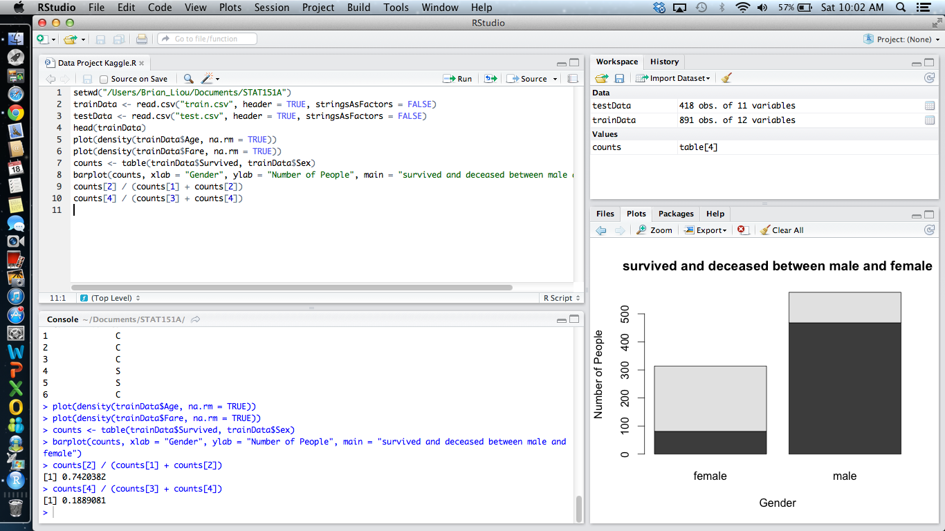
Note that in the barplot you create the lighter areas indicate survival. Doing the calculations below the barplot we see that in our Train data, 74.2% of women survived versus 18.9% of men.

Survival Rate by Passenger Class Barplot

Lets now look at the survival rate filtered by passenger class.

Pclass_survival <- table(trainData$Survived, trainData$Pclass)
barplot(Pclass_survival, xlab = "Cabin Class", ylab = "Number of People",
main = "survived and deceased between male and female")
Pclass_survival[2] / (Pclass_survival[1] + Pclass_survival[2])
Pclass_survival[4] / (Pclass_survival[3] + Pclass_survival[4])
Pclass_survival[6] / (Pclass_survival[5] + Pclass_survival[6])

It seems like the Pclass column might also be informative in survival prediction as the survival rate of the 1st class, 2nd class, and 3rd class are: 63.0%, 47.3%, and 24.2% respectively.

Though not covered, a few more insights would be useful here; survival rate based on fare rages, survival rate based on age ranges etc. The key idea is that we’re trying to determine if any/which of our variables are related to what we’re trying to predict: Survived

Conclusion

You have now successfully read in the data into R and done some preliminary data exploration. Move on to the second post to begin digging into the data by cleaning it so you can build your prediction model. Move on to Part Two Here!

If you want more practice data projects, be sure to check out http://www.teamleada.com